Galaxy Catalog Analysis Example: Void probability function
In this example, we’ll show how to calculate the void probability function: the probability that a randomly placed sphere has zero galaxies inside it, aka the VPF. We will also calculate the UPF, the probability that a random sphere has a number density less than some threshold value. See, e.g., Tinker et al 2008, and references therein.
There is also an IPython Notebook in the following location that can be used as a companion to the material in this section of the tutorial:
halotools/docs/notebooks/galcat_analysis/basic_examples/galaxy_catalog_analysis_tutorial8.ipynb
By following this tutorial together with this notebook, you can play around with your own variations of the calculation as you learn the basic syntax.
Generate a mock galaxy catalog
Let’s start out by generating a mock galaxy catalog into an N-body simulation in the usual way. Here we’ll assume you have the z=0 rockstar halos for the bolshoi simulation, as this is the default halo catalog.
from halotools.empirical_models import PrebuiltHodModelFactory
model = PrebuiltHodModelFactory('leauthaud11')
from halotools.sim_manager import CachedHaloCatalog
halocat = CachedHaloCatalog(simname = 'bolshoi', redshift = 0, halo_finder = 'rockstar')
model.populate_mock(halocat)
Our mock galaxies are stored in the galaxy_table of model.mock
in the form of an Astropy Table.
Extract the position and velocity coordinates
To calculate the mean radial velocity between two sets of points,
we need to know both their positions and velocities.
As described in Formatting your xyz coordinates for Mock Observables calculations,
functions in the mock_observables package
such as void_prob_func take array inputs in a
specific form: a (Npts, 3)-shape Numpy array. You can use the
return_xyz_formatted_array convenience
function for this purpose.
x = model.mock.galaxy_table['x']
y = model.mock.galaxy_table['y']
z = model.mock.galaxy_table['z']

from halotools.mock_observables import return_xyz_formatted_array
pos = return_xyz_formatted_array(x, y, z)
Calculate the VPF
To calculate the VPF, we need to specify the bins that define the sizes of the
randomly placed spheres, and we need to specify the number of spheres. Here will set
num_spheres to \(10^{5}\), but you should be sure to study the convergence
properties of this statistic on your galaxy sample as part of your study.
from halotools.mock_observables import void_prob_func

rbins = np.logspace(-1, 1.5, 20)
num_spheres = int(1e5)

vpf = void_prob_func(pos, rbins, num_spheres, period=model.mock.Lbox)
Calculate the UPF
The UPF quantifies the likelihood that a randomly places sphere contains
a number density below a given threshold. When calculating the UPF with
the underdensity_prob_func function,
this threshold density is defined as the number u times the
number density of the sample.
from halotools.mock_observables import underdensity_prob_func

u = 0.2
upf = underdensity_prob_func(pos, rbins, num_spheres, period=model.mock.Lbox, u=u)
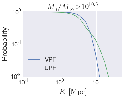
Plot the results
from seaborn import plt

plt.plot(rbins, vpf, label='VPF')
plt.plot(rbins, upf, label='UPF')

plt.xlim(xmin = 0.1, xmax = 50)
plt.ylim(ymin = 0.01, ymax = 1.1)
plt.loglog()
plt.xticks(fontsize=20)
plt.yticks(fontsize=20)
plt.xlabel(r'$R $  $\rm{[Mpc]}$', fontsize=25)
plt.ylabel('Probability', fontsize=25)
plt.legend(loc=3, fontsize=20)
plt.title(r'$M_{\ast}/M_{\odot} > 10^{10.5}$', fontsize=25)