Galaxy Catalog Analysis Example: Cluster BCG radial velocity dispersion profile
In this example we’ll show how to calculate the pairwise radial velocity
dispersion of galaxies relative to cluster BCGs,
\(\sigma_{\rm rad}^{2}(r)\).
In particular, we’ll use the Behroozi10SmHm model
to paint stellar masses onto subhalos, and then we’ll select a
population of \(M_{\ast}/M_{\odot}>10^{11.75}\) galaxies as our BCG sample,
and \(10^{10.75}<M_{\ast}/M_{\odot}<10^{11}\) galaxies as the
population we’ll use as tracers of the velocity field.
There is also an IPython Notebook in the following location that can be used as a companion to the material in this section of the tutorial:
halotools/docs/notebooks/galcat_analysis/basic_examples/galaxy_catalog_analysis_tutorial7.ipynb
By following this tutorial together with this notebook, you can play around with your own variations of the calculation as you learn the basic syntax.
Generate a mock galaxy catalog
Let’s start out by generating a mock galaxy catalog into an N-body simulation in the usual way. Here we’ll assume you have the z=0 rockstar halos for the bolshoi simulation, as this is the default halo catalog.
from halotools.empirical_models import PrebuiltSubhaloModelFactory
model = PrebuiltSubhaloModelFactory('smhm_binary_sfr')
from halotools.sim_manager import CachedHaloCatalog
halocat = CachedHaloCatalog(simname = 'multidark', redshift = 0, halo_finder = 'rockstar')
model.populate_mock(halocat)
Our mock galaxies are stored in the galaxy_table of model.mock
in the form of an Astropy Table.
Extract the position and velocity coordinates
To calculate the mean radial velocity between two sets of points,
we need to know both their positions and velocities.
As described in Formatting your xyz coordinates for Mock Observables calculations,
functions in the mock_observables package
such as radial_pvd_vs_r take array inputs in a
specific form: a (Npts, 3)-shape Numpy array. You can use the
return_xyz_formatted_array convenience
function for this purpose, which we will do after first
selecting a tracer and a BCG population of mock galaxies.
from halotools.mock_observables import return_xyz_formatted_array

cluster_central_mask = (model.mock.galaxy_table['stellar_mass'] > 10**11.75)
cluster_centrals = model.mock.galaxy_table[cluster_central_mask]

cluster_pos = return_xyz_formatted_array(cluster_centrals['x'],
    cluster_centrals['y'] ,cluster_centrals['z'])
cluster_vel = return_xyz_formatted_array(cluster_centrals['vx'],
    cluster_centrals['vy'] ,cluster_centrals['vz'])

low_mass_tracers_mask = ((model.mock.galaxy_table['stellar_mass'] > 10**10.75) &
                         (model.mock.galaxy_table['stellar_mass'] < 10**11))
low_mass_tracers = model.mock.galaxy_table[low_mass_tracers_mask]

low_mass_tracers_pos = return_xyz_formatted_array(low_mass_tracers['x'],
    low_mass_tracers['y'] ,low_mass_tracers['z'])
low_mass_tracers_vel = return_xyz_formatted_array(low_mass_tracers['vx'],
    low_mass_tracers['vy'] ,low_mass_tracers['vz'])
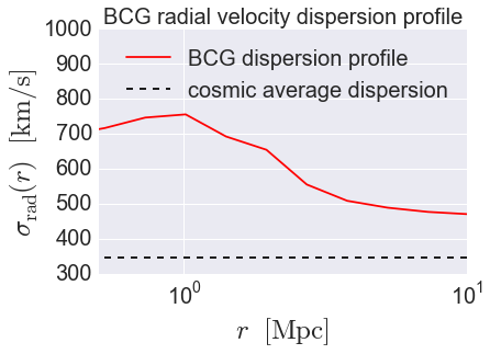
Calculate \(\sigma_{\rm rad}(r)\)
from halotools.mock_observables import radial_pvd_vs_r

rbins = np.logspace(-0.5, 1.5, 15)
rbin_midpoints = (rbins[1:] + rbins[:-1])/2.

vdisp_clusters = radial_pvd_vs_r(cluster_pos, cluster_vel, rbins,
                    sample2=low_mass_tracers_pos, velocities2=low_mass_tracers_vel,
                    period = model.mock.Lbox, do_auto=False, do_cross=True)

cosmic_avg = np.std(low_mass_tracers_vel[:,2])
Plot the result
from seaborn import plt

plt.plot(rbin_midpoints, vdisp_clusters, color='red',
         label = 'BCG dispersion profile')
plt.plot(np.logspace(-2, 5, 100), np.zeros(100)+cosmic_avg, '--', color='k',
         label = 'cosmic average dispersion')

plt.xscale('log')
plt.xlim(xmin = 0.5, xmax=10)
plt.ylim(ymin = 300, ymax = 1000)
plt.xticks(fontsize=20)
plt.yticks(fontsize=20)
plt.xlabel(r'$r $  $\rm{[Mpc]}$', fontsize=25)
plt.ylabel(r'$\sigma_{\rm rad}(r)$  $[{\rm km/s}]$', fontsize=25)
plt.title('BCG radial velocity dispersion profile', fontsize=20)
plt.legend(fontsize=20, loc='best')