Modeling Halo Spin-Dependent Disk-to-Bulge Mass Ratios

In this example, we will show how to use Conditional Abundance Matching to build a very simple model for \(B/T\), the bulge-to-total stellar mass ratio. In this model, galaxies with increasing stellar mass become “bulgier”, and at fixed stellar mass, halos with low spin have bigger bulges than halos with large spin. While this model is physically simplistic, it demonstrates the flexibility of the technique beyond the log-normal distribution shown in the tutorial on Modeling Central Galaxy Luminosity with Assembly Bias. The code used to generate these results can be found here:

halotools/docs/notebooks/cam_modeling/cam_disk_bulge_ratios_demo.ipynb

Baseline model for B/T

As a first step in the modeling, we’ll use the Moster+13 model for the stellar-to-halo-mass relation to paint \(M_{\ast}\) onto every subhalo in Bolshoi:

from halotools.sim_manager import CachedHaloCatalog
halocat = CachedHaloCatalog()

from halotools.empirical_models import Moster13SmHm
model = Moster13SmHm()
halocat.halo_table['stellar_mass'] = model.mc_stellar_mass(
    prim_haloprop=halocat.halo_table['halo_mpeak'], redshift=0)

We will model the bulge-to-total mass ratio using a simple power law. The scipy.stats.powerlaw model accepts a single parameter, \(a\), regulating the slope of the distribution. This slope should behave so that as \(M_{\ast}\) increases, the distribution becomes more heavily weighted with bulge-dominated systems, i.e., with large values of \(B/T.\)

def powerlaw_index(log_mstar):
    abscissa = [9, 10, 11.5]
    ordinates = [3, 2, 1]
    return np.interp(log_mstar, abscissa, ordinates)

a = powerlaw_index(np.log10(halocat.halo_table['stellar_mass']))

We will generate a Monte Carlo realization of this model using the isf method of powerlaw. The isf method analytically evaluates the inverse CDF of the power law distribution, and so this method makes it straightforward to generate a Monte Carlo realization of the power law model via inverse transformation sampling.

Under normal applications of inverse transformation sampling with isf, you simply pass in a uniform random variable as the argument. However, as described in Basic Idea Behind CAM, we can generalize the inverse transformation sampling technique so that the modeled variable is not purely stochastic, but is instead correlated with some other variable. In this example, we will choose to correlate \(B/T\) with halo spin. To do so, we need to calculate \({\rm Prob}(<\lambda_{spin}\vert M_{\ast})\), which we can do using the sliding_conditional_percentile function.

from halotools.utils import sliding_conditional_percentile

x = halocat.halo_table['stellar_mass']
y = halocat.halo_table['halo_spin']
nwin = 201
halocat.halo_table['spin_percentile'] = sliding_conditional_percentile(x, y, nwin)

Now that the spin percentile has been calculated, we just pass this quantity to the isf function to get a realization of our model:

u = halocat.halo_table['spin_percentile']
halocat.halo_table['bulge_to_total_ratio'] = 1 - powerlaw.isf(1 - u, a)

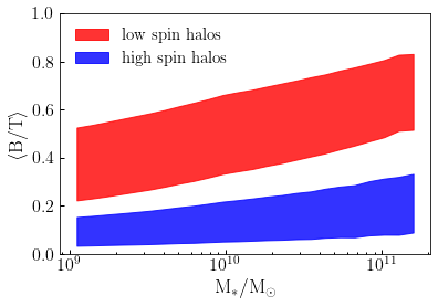
The plot below illustrates our results: