Modeling Central Galaxy Luminosity with Assembly Bias
In this example, we will show how to use Conditional Abundance Matching to map central galaxy luminosity onto halos in a way that simultaneously correlates with halo \(M_{\rm vir}\) and halo \(V_{\rm max}\). The code used to generate these results can be found here:
halotools/docs/notebooks/cam_modeling/cam_decorated_clf.ipynb
Baseline mass-to-light model
The approach we will demonstrate in this tutorial is very similar to the ordinary Conditional Luminosity Function model (CLF) of central galaxy luminosity. In the CLF, a parameterized form is chosen for the median luminosity of central galaxies as a function of host halo mass. The code below shows how to calculate this median luminosity for every host halo in the Bolshoi simulation:
from halotools.sim_manager import CachedHaloCatalog
halocat = CachedHaloCatalog(simname='bolplanck')
host_halos = halocat.halo_table[halocat.halo_table['halo_upid']==-1]
from halotools.empirical_models import Cacciato09Cens
model = Cacciato09Cens()
host_halos['median_luminosity'] = model.median_prim_galprop(
    prim_haloprop=host_halos['halo_mvir'])
To generate a Monte Carlo realization of the model,
one typically assumes that luminosities are distributed
as a log-normal distribution centered about this median relation.
While there is already a convenience function
mc_prim_galprop for the
Cacciato09Cens class that handles this,
it is straightforward to do this yourself
using the norm function in scipy.stats.
You just need to generate uniform random numbers and pass the result to the
scipy.stats.norm.isf function:
from scipy.stats import norm
loc = np.log10(host_halos['median_luminosity'])
uran = np.random.rand(len(host_halos))
host_halos['luminosity'] = 10**norm.isf(1-uran, loc=loc, scale=0.2)
The isf function analytically evaluates the inverse CDF of the normal distribution,
and so this Monte Carlo method is based on inverse transformation sampling.
It is probably more common to use numpy.random.normal for this purpose,
but doing things with scipy.stats.norm will make it easier
to see how CAM works in the next section.
Correlating scatter in luminosity with halo \(V_{\rm max}\)
As described in Basic Idea Behind CAM, we can generalize the inverse transformation sampling
technique so that the modeled variable is not purely stochastic, but is instead
correlated with some other variable. In this example, we will choose to
correlate the scatter with \(V_{\rm max}\). To do so, we need to calculate
\({\rm Prob}(<V_{\rm max}\vert M_{\rm vir})\), which we can do using
the sliding_conditional_percentile function.
from halotools.utils import sliding_conditional_percentile
x = host_halos['halo_mvir']
y = host_halos['halo_vmax']
nwin = 301
host_halos['vmax_percentile'] = sliding_conditional_percentile(x, y, nwin)
Now that \({\rm Prob}(<V_{\rm max}\vert M_{\rm vir})\) has been calculated,
we simply use these values instead of uniform randoms as the argument to the
scipy.stats.norm.isf function. This way, below-average values of \(V_{\rm max}\)
will be assigned below-average values of luminosity, and conversely.
loc = np.log10(host_halos['median_luminosity'])
u = host_halos['vmax_percentile']
host_halos['luminosity'] = 10**norm.isf(1-u, loc=loc, scale=0.2)
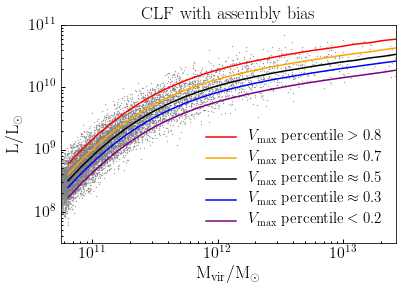
The plot below illustrates our results. The gray points show the Monte Carlo realization of central galaxy luminosity as a function of host halo mass. Each of the different curves shows the median relation calculated for halos with different values of \(V_{\rm max}\).