Modeling Complex Star-Formation Rates

In this example, we will show how to use Conditional Abundance Matching to model a correlation between the mass accretion rate of a halo and the specific star-formation rate of the galaxy living in the halo. The code used to generate these results can be found here:

halotools/docs/notebooks/cam_modeling/cam_complex_sfr_tutorial.ipynb

Observed star-formation rate distribution

We will work with a distribution of star-formation rates that would be difficult to model analytically, but that is well-sampled by some observed galaxy population. The particular form of this distribution is not important for this tutorial, since our CAM application will directly use the “observed” population to define the distribution that we recover.

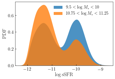
The plot above shows the specific star-formation rates of the toy galaxy distribution we have created for demonstration purposes. Briefly, there are separate distributions for quenched and star-forming galaxies. For the quenched galaxies, we model sSFR using an exponential power law; for star-forming galaxies, we use a log-normal; implementation details can be found in the notebook.

Modeling sSFR with CAM

We will start out by painting stellar mass onto subhalos in the Bolshoi simulation, which we do using the stellar-to-halo mass relation from Moster et al 2013.

from halotools.sim_manager import CachedHaloCatalog
halocat = CachedHaloCatalog()

from halotools.empirical_models import Moster13SmHm
model = Moster13SmHm()

halocat.halo_table['stellar_mass'] = model.mc_stellar_mass(
    prim_haloprop=halocat.halo_table['halo_mpeak'], redshift=0)

Algorithm description

We will now use CAM to paint star-formation rates onto these model galaxies. The way the algorithm works is as follows. For every model galaxy, we find the observed galaxy with the closest stellar mass. We set up a window of ~200 observed galaxies bracketing this matching galaxy; this window defines \({\rm Prob(< sSFR | M_{\ast})}\), which allows us to calculate the rank-order sSFR-percentile for each galaxy in the window. Similarly, we set up a window of ~200 model galaxies; this window defines \({\rm Prob(< dM_{vir}/dt | M_{\ast})}\), which allows us to calculate the rank-order accretion-rate-percentile of our model galaxy, \(r_1\). Then we simply search the observed window for the observed galaxy whose rank-order sSFR-percentile equals \(r_1\), and map its sSFR value onto our model galaxy. We perform that calculation for every model galaxy with the following syntax:

from halotools.empirical_models import conditional_abunmatch
x = halocat.halo_table['stellar_mass']
y = halocat.halo_table['halo_dmvir_dt_100myr']
x2 = galaxy_mstar
y2 = np.log10(galaxy_ssfr)
nwin = 201
halocat.halo_table['log_ssfr'] = conditional_abunmatch(x, y, x2, y2, nwin)

Results

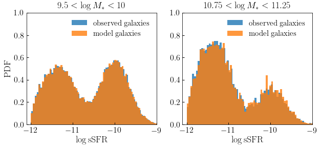
Now let’s inspect the results of our calculation. First we show that the distribution specific star-formation rates of our model galaxies matches the observed distribution across the range of stellar mass:

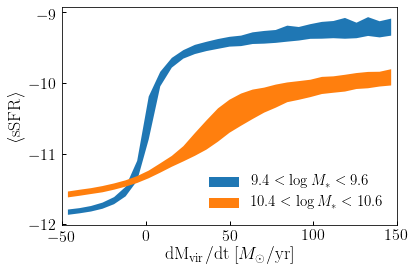
Next we can see that these sSFR values are tightly correlated with halo accretion rate at fixed stellar mass: