noisy_percentile

halotools.empirical_models.noisy_percentile(percentile, correlation_coeff, seed=None, random_percentile=None)

Starting from an input array storing the rank-order percentile of some quantity, add noise to these percentiles to achieve the desired Spearman rank-order correlation coefficient between percentile and noisy_percentile.

Parameters:

percentilendarray

Numpy array of shape (npts, ) storing values between 0 and 1, exclusive.

correlation_coefffloat or ndarray

Float or ndarray of shape (npts, ) storing values between 0 and 1, inclusive.

seedint, optional

Random number seed used to introduce noise

random_percentile: ndarray, optional

Numpy array of shape (npts, ) storing pre-computed random percentiles that will be used to mix with the input percentile. Default is None, in which case the random_percentile array will be automatically generated as uniform randoms according to the input seed.

Returns:

noisy_percentilendarray

Numpy array of shape (npts, ) storing an array such that the Spearman rank-order correlation coefficient between percentile and noisy_percentile is equal to the input correlation_coeff.

Notes

The plot below shows how the noisy_percentile function adds stochasticity to the input percentile: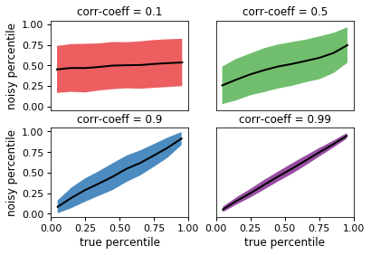

In the top-left panel, the correlation_coeff argument has been set to 0.1, so that there is only a weak correlation between the input percentile and the returned result. Conversely, in the bottom-right panel, the correlation is very tight.

Because the noisy_percentile function is so general, there are many variations on how you can use it to model correlations between galaxy and halo properties. Many such applications are based on the method of inverse transformation sampling to generate Monte Carlo realizations of galaxy properties, and so the halotools.utils.monte_carlo_from_cdf_lookup function and the halotools.utils.build_cdf_lookup function may come in handy.

In the Examples section below, we demonstrate how you can implement a correlation between halo concentration and scatter in the stellar-to-halo mass relation. In this particular case, we will use a log-normal PDF for the distribution of \(M_\ast\) at fixed halo mass. Note, however, that the noisy_percentile function does not require that the statistical distribution of the galaxy property being modeled necessarily have any particular functional form. So long as you have knowledge of the rank-order percentile of your galaxy property, noisy_percentile allows you to introduce correlations of arbitrary strength with any other variable for which you also know the rank-order percentile.

Also see Tutorial on Conditional Abundance Matching demonstrating how to use this function in galaxy-halo modeling with several worked examples.

Examples

The noisy_percentile function is useful as the kernel of a calculation in which you are modeling a correlation between a galaxy property and some halo property. For example, suppose you have a sample of halos at fixed mass, and you want to map stellar mass onto the halos according to a log-normal distribution, such that the scatter in \(M_{\ast}\) is correlated with halo concentration. The code below shows how to use the noisy_percentile function for this purpose, together with the scipy implementation of a Gaussian PDF, norm.

In the demo below, we’ll start out by selecting a sample of halos at fixed mass using a fake halo catalog that is generated on-the-fly; note that the API would be the same for any CachedHaloCatalog.

>>> from halotools.sim_manager import FakeSim
>>> halocat = FakeSim()
>>> mask = (halocat.halo_table['halo_mpeak'] > 10**11.9)
>>> mask *= (halocat.halo_table['halo_mpeak'] < 10**12.1)
>>> halo_sample = halocat.halo_table[mask]
>>> num_sample = len(halo_sample)

If we just wanted random uncorrelated scatter in stellar mass, we can pass the isf function a set of random uniform numbers:

>>> from scipy.stats import norm
>>> mean_logmstar, std_logmstar = 11, 0.1
>>> uran = np.random.rand(num_sample)
>>> mstar_random = norm.isf(uran, loc=mean_logmstar, scale=std_logmstar)

The mstar_random array is just a normal distribution in \(\log_{10}M_\ast\), with deviations from the mean value of 11 being uncorrelated with anything. To implement a correlation between \(M_\ast - \langle M_{\ast}\rangle\) and concentration, we first calculate the rank-order percentile of the concentrations of our halo sample, simply by sorting and normalizing by the number of objects:

>>> from halotools.utils import rank_order_percentile
>>> percentile = rank_order_percentile(halo_sample['halo_nfw_conc'])

If we wanted to implement a perfect correlation between concentration and scatter in \(M_\ast\), with lower concentrations receiving lower stellar mass, we would just pass the array 1 - percentile to the isf function:

>>> mstar_maxcorr = norm.isf(1-percentile, loc=mean_logmstar, scale=std_logmstar)

The noisy_percentile function allows you to build correlations of a strength that is intermediate between these two extremes. If you want \(M_\ast\) and concentration to have a Pearson correlation coefficient of 0.5:

>>> correlation_coeff = 0.5
>>> result = noisy_percentile(percentile, correlation_coeff)
>>> mstar_0p5 = norm.isf(1-result, loc=mean_logmstar, scale=std_logmstar)

In the figure below, we visually demonstrate the results of this calculation by showing the PDF of \(\log_{10}M_\ast\) for our halo sample, color-coded by the mean concentration of the halos with a given stellar mass:

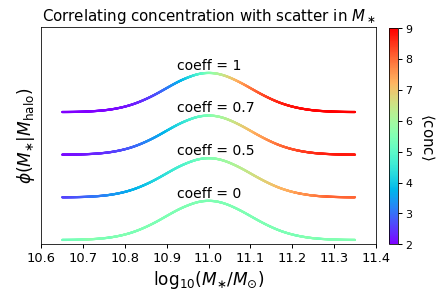
For each of the different curves, the overall normalization of \(\phi(M_{\ast})\) has been offset for clarity. For the case of a correlation coefficient of unity (the top curve), we see that halos with above-average \(M_\ast\) values for their mass tend to have above-average concentration values for their mass, and conversely for halos with below-average \(M_\ast\). For the case of zero correlation (the bottom curve), there is no trend at all. Correlation strengths between zero and unity span the intermediary cases.