Halo Catalog Analysis Example: calculating radial profiles

In this example, we’ll show how to start from a subhalo catalog and calculate how various halo properties vary as a function of 3d distance from some nearby halo, i.e. we’ll show how to use Halotools to calculate radial profiles. In particular, we’ll see how the radial_profile_3d function can be used to show that the mass accretion rate of halos decreases as those halos approach a nearby cluster. We’ll also show how to calculate the mean number density of some sample as a function of cluster-centric distance.

Before following this tutorial, make sure you understand Halo Catalog Analysis Example: halo properties as a function of host halo mass, as that tutorial covers basic material such as how halo data is organized into an Astropy Table object.

There is also an IPython Notebook in the following location that can be used as a companion to the material in this section of the tutorial:

halotools/docs/notebooks/halocat_analysis/basic_examples/halo_catalog_analysis_tutorial2.ipynb

By following this tutorial together with this notebook, you can play around with your own variations of the calculation as you learn the basic syntax.

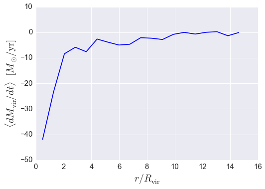
Example 1: \(dM_{\rm vir}/dt\) vs. halo-centric distance

Let’s start out by selecting two samples of halos from the Bolshoi simulation: one sample of group-mass host halos, and a second sample of lower-mass halos.

Note that the lower-mass sample includes subhalos since we do not make a halo_upid cut.

from halotools.sim_manager import CachedHaloCatalog
halocat = CachedHaloCatalog(simname = 'bolshoi', redshift = 0)

host_mask = ((halocat.halo_table['halo_upid'] == -1) &
                (halocat.halo_table['halo_mvir'] > 1e13) &
                (halocat.halo_table['halo_mvir'] < 2e13))
group_mass_hosts = halocat.halo_table[host_mask]

low_mass_mask = ((halocat.halo_table['halo_mpeak'] > 5e11) &
                (halocat.halo_table['halo_mpeak'] < 6e11))
low_mass_halos = halocat.halo_table[low_mass_mask]

The first question we will ask of these is halos is the following: how does the mass accretion rate of (sub)halos vary as a function of the distance to the group-mass hosts?

As with all mock_observables functions that accept 3d positions for arguments, we first format our positions into an array of the expected shape.

from halotools.mock_observables import return_xyz_formatted_array

group_mass_hosts_pos = return_xyz_formatted_array(group_mass_hosts['halo_x'], group_mass_hosts['halo_y'], group_mass_hosts['halo_z'])
low_mass_halos_pos = return_xyz_formatted_array(low_mass_halos['halo_x'], low_mass_halos['halo_y'], low_mass_halos['halo_z'])

The radial_profile_3d function accepts two different kinds of inputs for the separation bins. If you pass in rbins_normalized and normalize_rbins_by, then this combination of arguments allows you to calculate how various quantities vary as a function of, for example, \(x = r / R_{\rm vir}.\) The way this works is that the normalize_rbins_by argument stores the value of \(R_{\rm vir}\) for each point in sample1, and the rbins_normalized argument will be interpreted as referring to the distance of points in sample2 scaled by this value.

In the following call to the radial_profile_3d function, we will calculate the mean mass accretion rate of the lower-mass halos in 20 bins linearly spaced between \(0.1 < r / R_{\rm vir} < 15.\)

from halotools.mock_observables import radial_profile_3d

rbins_normalized = np.linspace(0.1, 15, 20)
rbins_midpoints = (rbins_normalized[:-1] + rbins_normalized[1:])/2.

result = radial_profile_3d(group_mass_hosts_pos, low_mass_halos_pos, low_mass_halos['halo_dmvir_dt_tdyn'],
                           rbins_normalized = rbins_normalized,
                           normalize_rbins_by = group_mass_hosts['halo_rvir'],
                           period=halocat.Lbox)

plt.plot(rbins_midpoints, result, color='blue')

plt.xlabel(r'$r / R_{\rm vir}$', fontsize=20)
plt.ylabel(r'$\langle dM_{\rm vir} / dt \rangle$  $[M_{\odot}/{\rm yr}]$', fontsize=20)
plt.xticks(size=15); plt.yticks(size=15)

As we’ll see in the next example, if you instead want to calculate the profile of a quantity as a function of the absolute distance rather than some scaled distance, you can use the rbins_absolute argument instead.

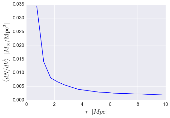
Example 2: Number density vs host-centric distance

In this next example, we’ll calculate the answer to the following question: how does the abundance of (sub)halos vary as a function of host-centric distance to our sample of group-mass host halos?

The radial_profile_3d function has a return_counts argument that can be used to additionally return the number of objects as a function of the input distance. In the following call to the radial_profile_3d function, we will calculate the mean mass accretion rate of the lower-mass halos in 20 bins linearly spaced in r between \(0.5 {\\rm Mpc} < r < 10 {\\rm Mpc}.\)

rbins_absolute = np.linspace(0.5, 10, 20)
rbins_midpoints = (rbins_absolute[:-1] + rbins_absolute[1:])/2.

result, counts = radial_profile_3d(group_mass_hosts_pos, low_mass_halos_pos, low_mass_halos['halo_dmvir_dt_tdyn'],
                           rbins_absolute = rbins_absolute,
                           period=halocat.Lbox, return_counts = True)

shell_volumes = 4*np.pi*(rbins_midpoints**2)*np.diff(rbins_absolute)
mean_number_density = (counts/float(len(group_mass_hosts)))/shell_volumes

plt.plot(rbins_midpoints, mean_number_density, color='blue')

plt.xlabel(r'$r$  $[Mpc]$', fontsize=20)
plt.ylabel(r'$\langle dN/dV \rangle$  $[M_{\odot}/{\rm Mpc^{3}}]$', fontsize=20)
plt.xticks(size=15); plt.yticks(size=15)