Galaxy Catalog Analysis Example: Galaxy properties as a function of halo mass
In this example, we’ll show how to start from a sample of mock galaxies and calculate how various galaxies properties scale with halo mass. In particular, we’ll calculate the average total stellar mass, \(\langle M_{\ast}^{\rm tot}\vert M_{\rm halo}\rangle\), and also the average quiescent fraction for centrals and satellites, \(\langle F_{\rm cen}^{\rm q}\vert M_{\rm halo}\rangle\) and \(\langle F_{\rm sat}^{\rm q}\vert M_{\rm halo}\rangle\).
There is also an IPython Notebook in the following location that can be used as a companion to the material in this section of the tutorial:
halotools/docs/notebooks/galcat_analysis/basic_examples/galaxy_catalog_analysis_tutorial1.ipynb
By following this tutorial together with this notebook, you can play around with your own variations of the calculation as you learn the basic syntax.
Generate a mock galaxy catalog
Let’s start out by generating a mock galaxy catalog into an N-body simulation in the usual way. Here we’ll assume you have the z=0 rockstar halos for the bolshoi simulation, as this is the default halo catalog.
from halotools.empirical_models import PrebuiltSubhaloModelFactory
model = PrebuiltSubhaloModelFactory('smhm_binary_sfr')
from halotools.sim_manager import CachedHaloCatalog
halocat = CachedHaloCatalog(simname = 'bolshoi', redshift = 0, halo_finder = 'rockstar')
model.populate_mock(halocat)
Now suppose the data we are interested in is complete for
\(M_{\ast} > 10^{10}M_{\odot},\) so we will make a cut on the mock.
Our mock galaxies are stored in the galaxy_table of model.mock
in the form of an Astropy Table.
sample_mask = model.mock.galaxy_table['stellar_mass'] > 1e10
gals = model.mock.galaxy_table[sample_mask]
Calculate total stellar mass \(M_{\ast}^{\rm tot}\) in each halo
To calculate the total stellar mass of galaxies in each halo, we’ll use
the halotools.utils.group_member_generator. You can read more about the
details of that function in its documentation, here we’ll just demo some basic usage.
Briefly, this generator can be used to iterate over your galaxy population
on a group-by-group basis, so that you can perform group-wise calculations
with each step of the iteration. In this case, at each step of the iteration
we’ll sum up the stellar masses of each group’s members.
The halo_hostid is a natural grouping key for a galaxy catalog whose
host halos are known. So we’ll sort our galaxy catalog on this column,
notify the group_member_generator that we have done so
by passing in halo_hostid as the grouping_key, and then request that
the generator yield the data stored in the stellar_mass column
at each iteration. The we’ll loop over the generator,
calculate the sum of the yielded stellar mass column,
and broadcast the result to each group member.
from halotools.utils import group_member_generator

gals.sort('halo_hostid')
grouping_key = 'halo_hostid'
requested_columns = ['stellar_mass']
group_gen = group_member_generator(gals, grouping_key, requested_columns)

total_stellar_mass = np.zeros(len(gals))
for first, last, member_props in group_gen:
    stellar_mass_of_members = member_props[0]
    total_stellar_mass[first:last] = sum(stellar_mass_of_members)

gals['halo_total_stellar_mass'] = total_stellar_mass
Our gals table now has a halo_total_stellar_mass column.
Calculate host halo mass \(M_{\rm host}\) of each galaxy
Now we’ll do a very similar calculation, but instead broadcasting the
host halo mass to each halo’s members. Here we’ll perform a two-property sort.
By sorting first on halo_hostid and then on halo_upid, what we accomplish is that
galaxies sharing a common halo are grouped together, and then within each grouping
the true central galaxy appears first in the sequence. This means that when the
group_member_generator yields arrays to us, we can retrieve the
property of the central galaxy via the first element in each yielded array.
In this next calculation, we’ll exploit that information to broadcast the
host halo virial mass to all members of the halo.
gals.sort(['halo_hostid', 'halo_upid'])
grouping_key = 'halo_hostid'
requested_columns = ['halo_mvir']
group_gen = group_member_generator(gals, grouping_key, requested_columns)

host_mass = np.zeros(len(gals))
for first, last, member_props in group_gen:
    mvir_members = member_props[0]
    mvir_host = mvir_members[0]
    host_mass[first:last] = mvir_host

gals['halo_mhost'] = host_mass
Our gals table now has a halo_mhost column.
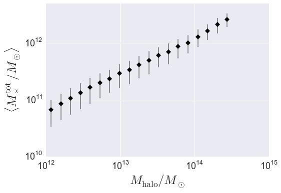
Calculate \(\langle M_{\ast}^{\rm tot}\rangle\) vs. \(M_{\rm halo}\)
Now we’ll exploit our previous calculations to compute the mean total stellar mass
in bins of halo mass. For this calculation,
the mean_y_vs_x provides useful wrapper behavior around
scipy.stats.binned_statistic and numpy.histogram.
Note that mean_y_vs_x is really just a convenience
function used for quick exploratory work. For results going into science publications,
be sure to check how your findings depend on bin width, sampling, etc.
from halotools.mock_observables import mean_y_vs_x
import numpy as np

bins = np.logspace(12, 15, 25)
result = mean_y_vs_x(gals['halo_mhost'].data,
                     gals['halo_total_stellar_mass'].data,
                     bins = bins,
                     error_estimator = 'variance')

host_mass, mean_stellar_mass, mean_stellar_mass_err = result
Plot the result
from seaborn import plt

plt.errorbar(host_mass, mean_stellar_mass, yerr=mean_stellar_mass_err,
             fmt = "none", ecolor='gray')
plt.plot(host_mass, mean_stellar_mass, 'D', color='k')

plt.loglog()
plt.xticks(size=18)
plt.yticks(size=18)
plt.xlabel(r'$M_{\rm halo}/M_{\odot}$', fontsize=25)
plt.ylabel(r'$\langle M_{\ast}^{\rm tot}/M_{\odot}\rangle$', fontsize=25)
plt.ylim(ymax=5e12)
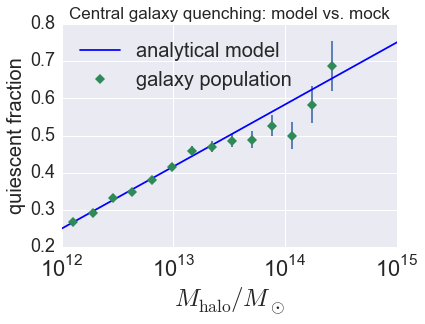
Quiescent fraction of centrals and satellites
In this section we’ll perform a very similar calculation to the above, only here we’ll compute the average quiescent fraction of centrals and satellites.
Calculate \(\langle F_{\rm q}^{\rm cen}\vert M_{\rm halo} \rangle\) and \(\langle F_{\rm q}^{\rm sat} \vert M_{\rm halo}\rangle\)
In the above calculation, we needed to create new columns for our galaxy catalog, \(M_{\rm host}\) and \(M_{\ast}^{\rm tot}\). Here we’ll reuse the \(M_{\rm host}\) column, and our model already created a boolean-valued quiescent column for our galaxies. So no group iteration is necessary; all we need to do is calculate the average trends as a function of halo mass.
cens_mask = gals['halo_upid'] == -1
cens = gals[cens_mask]
sats = gals[~cens_mask]

bins = np.logspace(12, 14.5, 15)

# centrals
result = mean_y_vs_x(cens['halo_mhost'].data, cens['quiescent'].data,
            bins = bins)
host_mass, fq_cens, fq_cens_err_on_mean = result

# satellites
result = mean_y_vs_x(sats['halo_mhost'].data, sats['quiescent'].data,
            bins = bins)
host_mass, fq_sats, fq_sats_err_on_mean = result
Plot the result and compare it to the underlying analytical relation
plt.errorbar(host_mass, fq_cens, yerr=fq_cens_err_on_mean,
             color='seagreen', fmt = "none")
plt.plot(host_mass, fq_cens, 'D', color='seagreen',
             label = 'galaxy population')

analytic_result_mhost_bins = np.logspace(10, 15.5, 100)
analytic_result_mean_quiescent_fraction = model.mean_quiescent_fraction(prim_haloprop = analytic_result_mhost_bins)
plt.plot(analytic_result_mhost_bins,
         analytic_result_mean_quiescent_fraction,
         color='blue', label = 'analytical model')

plt.xscale('log')
plt.xticks(size=22)
plt.yticks(size=18)
plt.xlabel(r'$M_{\rm halo}/M_{\odot}$', fontsize=25)
plt.ylabel('quiescent fraction', fontsize=20)
plt.xlim(xmin = 1e12, xmax = 1e15)
plt.ylim(ymin = 0.2, ymax=0.8)
plt.legend(frameon=False, loc='best', fontsize=20)
plt.title('Central galaxy quenching: model vs. mock', fontsize=17)
This tutorial continues with Galaxy Catalog Analysis Example: Calculating galaxy clustering in 3d.