Galaxy Catalog Analysis Example: Calculating galaxy clustering in 3d
In this example, we’ll show how to calculate the two-point clustering of a mock galaxy catalog, \(\xi_{\rm gg}(r)\). We’ll also show how to compute cross-correlations between two different galaxy samples, and also the one-halo and two-halo decomposition \(\xi^{\rm 1h}_{\rm gg}(r)\) and \(\xi^{\rm 2h}_{\rm gg}(r)\).
There is also an IPython Notebook in the following location that can be used as a companion to the material in this section of the tutorial:
halotools/docs/notebooks/galcat_analysis/basic_examples/galaxy_catalog_analysis_tutorial2.ipynb
By following this tutorial together with this notebook, you can play around with your own variations of the calculation as you learn the basic syntax.
Generate a mock galaxy catalog
Let’s start out by generating a mock galaxy catalog into an N-body simulation in the usual way. Here we’ll assume you have the z=0 rockstar halos for the bolshoi simulation, as this is the default halo catalog.
from halotools.empirical_models import PrebuiltSubhaloModelFactory
model = PrebuiltSubhaloModelFactory('smhm_binary_sfr')
from halotools.sim_manager import CachedHaloCatalog
halocat = CachedHaloCatalog(simname = 'bolshoi', redshift = 0, halo_finder = 'rockstar')
model.populate_mock(halocat)
Our mock galaxies are stored in the galaxy_table of model.mock
in the form of an Astropy Table.
Calculate two-point galaxy clustering \(\xi_{\rm gg}(r)\)
The three-dimensional galaxy clustering signal is calculated by
the tpcf function from
the x, y, z positions of the galaxies stored in the galaxy_table.
We can retrieve these arrays as follows:
x = model.mock.galaxy_table['x']
y = model.mock.galaxy_table['y']
z = model.mock.galaxy_table['z']
As described in Formatting your xyz coordinates for Mock Observables calculations,
functions in the mock_observables package
such as tpcf take array inputs in a
specific form: a (Npts, 3)-shape Numpy array. You can use the
return_xyz_formatted_array convenience
function for this purpose, which has a built-in mask feature
that we’ll also demonstrate to select positions of only those
galaxies with \(M_{\ast}>10^{10}M_{\odot}.\)
from halotools.mock_observables import return_xyz_formatted_array
sample_mask = model.mock.galaxy_table['stellar_mass'] > 1e10
pos = return_xyz_formatted_array(x, y, z, mask = sample_mask)
To calculate the clustering:
from halotools.mock_observables import tpcf

import numpy as np
rbins = np.logspace(-1, 1.25, 15)
rbin_centers = (rbins[1:] + rbins[:-1])/2.

xi_all = tpcf(pos, rbins, period = model.mock.Lbox, num_threads = 'max')
Decomposition into the 1-halo and 2-halo terms
The tpcf_one_two_halo_decomp function calculates the two-point
correlation function, decomposed into contributions from galaxies in the
same halo, and galaxies in different halos. In order to use this
function, we must provide an input array of host halo IDs that are equal
for galaxies occupying the same halo, and distinct for galaxies in
different halos. We’ll use the halo_hostid column for this purpose,
using the same sample_mask as above.
from halotools.mock_observables import tpcf_one_two_halo_decomp

halo_hostid = model.mock.galaxy_table['halo_hostid'][sample_mask]

xi_1h, xi_2h = tpcf_one_two_halo_decomp(pos,
                halo_hostid, rbins,
                period = model.mock.Lbox,
                num_threads='max')
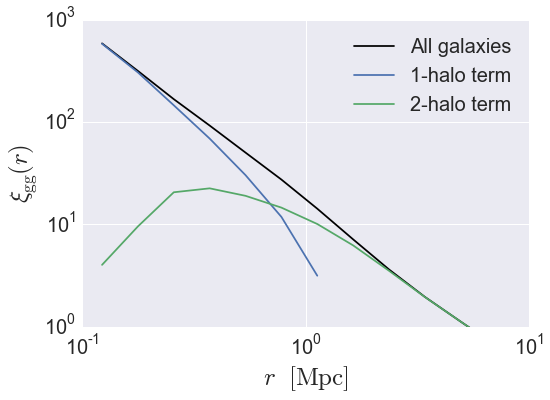
Plot the results
from seaborn import plt

plt.plot(rbin_centers, xi_all,
         label='All galaxies', color='k')
plt.plot(rbin_centers, xi_1h,
         label = '1-halo term')
plt.plot(rbin_centers, xi_2h,
         label = '2-halo term')

plt.xlim(xmin = 0.1, xmax = 10)
plt.ylim(ymin = 1, ymax = 1e3)
plt.loglog()
plt.xticks(fontsize=20)
plt.yticks(fontsize=20)
plt.xlabel(r'$r $  $\rm{[Mpc]}$', fontsize=25)
plt.ylabel(r'$\xi_{\rm gg}(r)$', fontsize=25)
plt.legend(loc='best', fontsize=20)
This tutorial continues with Galaxy Catalog Analysis Example: Galaxy-galaxy lensing.